Studying Studies: Part V – power and significance

If you’re thinking about digging into the scientific literature with the hope of finding some remarkable discoveries, but you’re worried that novel findings move at a glacial pace, fear not. According to John Ioannidis and his colleagues in JAMA in 2016, 96% of the biomedical literature report statistically significant results.¹Among 1.6 million abstracts and 385,393 full-text articles with p-values in MEDLINE (1990-2015), 96% reported at least one statistically significant result. “Significant discovery has become a boring nuisance,” Ioannidis says, in a Keynote address at the Lown Institute, in the same year. It’s therefore not hyperbolic to say that almost all scientific papers claim that they have found “significant” results.

So what does significant really mean in the scientific literature? Let’s backup slightly to answer this question.

The results of scientific papers are generally based on experiments. These experiments are statistical tests of hypotheses. A hypothesis is a fancy word for guess.²“Now, don’t laugh, that’s really true,” says Richard Feynman of the importance of this “guess” in science. One such example of a guess is: a compound first found in the soil on Easter Island, rapamycin, fed late in life, will extend the lifespan of mice.

In United States law, one is considered innocent until proven guilty as the default position. There is a presumption of innocence. The prosecution must prove, beyond a reasonable doubt, each essential element of the crime charged. Prosecutors bear the burden of proof.

In science, the default position in an experiment is that there is no relationship between two phenomena. This is called the null (i.e., zero) hypothesis. Therefore, in our example, the default presumption—the null hypothesis—is that rapamycin will not extend the lifespan of mice.

The investigators are like prosecutors, defendants, and judges rolled into one—which is why being impartial and unbiased are so critical to good science—they try to shoot down, or reject, the null hypothesis in a fair and rigorous manner. The null hypothesis is going to be accepted or rejected based on the results of the test, much like a defendant in a court case will be judged guilty or not guilty.

In the case of Rapamycin v. Lifespan, in perhaps an ironic twist, investigators are trying to determine if the compound is guilty of extending the lives of mice. The defendant, rapamycin, is presumed to be innocent (i.e., the null hypothesis is accepted) of this charge, until proven guilty (i.e, the null hypothesis is rejected) beyond a reasonable doubt (i.e., to a “statistically significant”³This is defined in more detail, below. degree).

In our example, brought to life in 2009 by Richard Miller and his group, rapamycin extends lifespan in mice when provided at 1.6 years of age, about 65 “mouse years old.” The null hypothesis that rapamycin will not extend the lives of mice is rejected and the alternative hypothesis that rapamycin increases lifespan is accepted in its place. (In neither case is the null hypothesis or its alternative proven, per se. Rather, the null hypothesis is tested with data and a decision is made based on how likely or unlikely the data are. Unlike in mathematics, there are no proofs in science.) Instead of a judge and jury, something called a p-value decides the fate of the guess. The verdict?

For data pooled across sites, a log-rank test rejected the null hypothesis that treatment and control groups did not differ (p < 0.0001); mice fed rapamycin were longer lived than controls (p < 0.0001) in both males and females. Expressed as mean lifespan, the effect sizes were 9% for males and 13% for females in the pooled dataset. Expressed as life expectancy at 600 days (the age of first exposure to rapamycin), the effect sizes were 28% for males and 38% for females.

In this case, we see that “p < 0.0001.” What does it mean that the p-value is less than 0.0001? The p-value (i.e., probability value) quantifies the degree of significance. The p-value is trying to answer the question: What is the probability—0 being that it is impossible and 1 being that it is certain—of rejecting the null hypothesis when it is, in fact, true? Asked another way, what is the probability that the effect (i.e., the difference between the groups) you are seeing is not due to the effect of rapamycin versus that of placebo, but instead is due to noise, or chance?

In other words, the investigators observed a difference—in which, if we supposed there truly was zero effect from rapamycin on lifespan—the probability of seeing a difference at least as extreme as their results is less than 1-in-10,000.

The higher the p-value, the greater the chance that the effect you are seeing is not real (i.e., the results seen are the result of chance), and the more the results support the null hypothesis. The lower the p-value, the greater the chance that the effect you are seeing is indeed real, and the less the results support the null hypothesis.

The result is deemed to be (or not to be, as it were) statistically significant based on a significance level that is preselected (i.e., before the study) by the investigators. This level is typically set at or below 5%. The significance level is also referred to as alpha, or α, where α is the probability of a false positive. (Ok, so at least one nice overlap between science and mathematics is the penchant for using Greek letters, though we get to use all of ‘em in math…not so much in science.)

If the p-value is less than 0.05, or 5%, the results are deemed “statistically significant.” If not, the results are deemed not statistically significant, and the null hypothesis is accepted.

In the rapamycin example, the observed p-value is less than 0.0001, or 0.01%, thus the result is statistically significant by any reasonable p-value cutoff.

When the investigators set a 5% significance level, they’re saying that they will accept anything less than a 5% risk of concluding that a difference exists when there is no actual difference. This is also called a false positive (i.e., detecting something that isn’t really there).

How confident should we be in confidence intervals?

The flipside of the significance level is called the confidence level. It’s 1 – α (i.e., significance level), so if the significance level is 0.05, the corresponding confidence level is 0.95 or 95%.

If you’ve read a few studies, or even a few abstracts in particular, you’ve undoubtedly seen confidence intervals (CIs). Often, you’ll see something like “1.17, 95% CI (1.05-1.31).” In this particular case, we’re looking at the associated risk between colorectal cancer and 100-gram-intake of red meat per day, from a 2011 meta-analysis of 10 observational studies. This was a statistically significant difference. We can determine that at a glance by looking at the CI and checking to see if it crosses 1.00. In this case it doesn’t, and we know that it’s a positive association because the numbers are greater than one. The “1.17” represents the result that a person eating 100 grams of red meat had an associated 17% increase in risk (i.e., a 1.17-fold increase) of colorectal cancer. Likewise, if the observed relative risk was less than 1.00, it would be a negative association. For example, if the results showed “0.89, 95% CI (0.77-1.07),” it would be a negative association–in this case it would represent an 11% associated decrease (i.e., 1 – 0.89) in risk–though one that is not statistically significant because the CI crossed 1.00.

It’s important to note that the CI (e.g., 95%) is not the probability that a specific confidence interval contains the population parameter. For example, many people think that we can be 95% confident that the true effect of increased meat consumption and colorectal cancer is between 1.05-1.31, but that’s not what the CI suggests.

If we were to take 100 different samples and compute a 95% CI for each sample, then approximately 95 of the 100 CIs will contain the true mean value. In practice, however, we select one random sample and generate one CI, which may or may not contain the true mean. A 95% CI says that 95% of experiments exactly like the one we just did will include the true mean, but 5% won’t. So there is a 1-in-20 chance (5%) that our CI does NOT include the true mean. CI is just as much a measure of uncertainty as it is of “confidence.” (Andrew Gelman, director of the Applied Statistics Center at Columbia and keeper of a thoughtful blog, prefers the term “uncertainty intervals” over confidence intervals. “The uncertainty interval tells you how much uncertainty you have.”)

Statistical significance vs. practical significance

If you recall, about 96% of scientific papers report statistical significance, so most papers pulled from the biomedical literature are bound to be a discovery of significance. (Astute readers of the Studying Studies series will recall that most of these findings turn out to be false, as Ioannidis has famously pointed out.) The word significant connotes meaning. But there can be a wide gap between statistical and practical meaning. Statistical significance says nothing about practical significance, though this fact is lost on many, especially those reporting on findings.

These two can be aligned, but often they are opposed to one another. In other words, something can be practically meaningful, but not statistically significant. Likewise, statistical significance, but practical irrelevance, can also occur.

One note of caution before we proceed: we allude to, but don’t take head-on, the high amount of data dredging (other terms for it include: p-hacking, fishing expeditions, researcher degrees of freedom, gardens of forking paths) that can occur where investigators somewhat naturally look hard for statistically significant results in their data, but this data doesn’t represent anything relevant to the general population. In other words, if the data is just noise (the null hypothesis is true), your chance of finding something “statistically significant” is a lot more than 5% because of this data dredging. In such cases, always look for the Bonferroni correction which raises the bar on significance by forcing the investigators to divide the p-value by the number of “looks” they take at the data. So, if the p-value is set at 0.05, but the investigators look at 20 different hypotheses, because the chances go up that they will find something significant, the p-value is divided by the number of looks (20), such that the hurdle for significance is now 0.0025 (0.05/20). Otherwise, even if investigators are looking at nothing but noise, the 0.05 p-value is actually telling us we should expect to see one of those 20 looks to have statistical significance (Figure 1).⁴A 5% chance is a 1-in-20 chance.

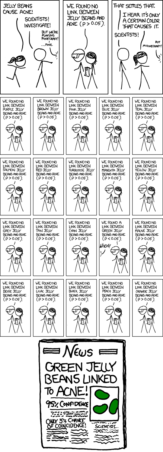
Figure 1. Significant?

Image credit: xkcd.com

Back to the practical matter. When is a study most commonly not statistically significant, but practically relevant? When a study doesn’t have enough patients to detect a “statistical” effect, but the difference between groups—the effect size—is relatively large.

What can one conclude, for example, from the results of a study looking at the effectiveness of a drug on lowering blood pressure when the p-value was greater than the significance level? The knee-jerk answer is that the result was not statistically significant, so the drug does not lower blood pressure. This is partially correct. It’s true that the drug did not have a statistically significant effect in the experiment, but unless you know what the observable differences were between the groups, how many subjects were in the study, and what the preselected significance level was, you don’t know if the drug helps lower blood pressure.

Nevertheless, the investigator accepts the null hypothesis for the experiment (and, as we learned, the likelihood of the test getting published also may be null!). However, there could be a Type II error (i.e., a false negative). In other words, the investigator may have failed to reject the null hypothesis when a genuine effect was there (Figure 2). The investigator may not have had an adequate number of subjects to detect a statistical difference between the two groups, when the observed differences might be 15 mmHg in systolic blood pressure, on average. The investigator may have preselected an especially stringent significance level, say, 0.005⁵Ioannidis and colleagues have proposed just this: changing the p-value threshold significance from 0.05 to 0.005 for novel discovery claims. instead of the typical 0.05.

On the other side of the spectrum, what can one determine, for example, from the results of a study looking at a different drug with the same purpose of lowering blood pressure when the p-value is less than the significance level?

If you happened to get through the previous paragraphs, you know this is almost a trick question. Yes, we can say that the results are statistically significant. But we can’t say whether this is of practical significance until we look at the magnitude of the observed effect, the number of subjects in the study, and the preselected significance level. For example, the study may have too many—yes, too many—subjects. Tests of this nature run the risk of generating statistical significance, but are practically insignificant. Just because the p-value is low, and therefore “statistically significant,” the result may be largely unimportant. The larger the N, the larger the probability the study will reach statistical significance with ever-declining differences between the groups in the study. If a study finds a drug that lowers systolic blood pressure by 0.1 mmHg, who cares? It’s not clinically relevant. But a large enough study will likely find this result, even if it tests a placebo versus another placebo.

To encapsulate these points, if a study was not statistically significant, we should always ask two questions:

1. What magnitude of difference (i.e., effect) was the study powered to detect?
2. Is it possible the effect was present, but not at the power threshold?

If a study was statistically significant, we should also ask two questions:

1. How big is the effect (i.e., the magnitude of difference between groups)?
2. How many people did you look at to detect the effect?

The latter two questions can almost assuredly be answered by looking at a table from the study, or even in the abstract. But how do we know what magnitude of difference the study was designed to pick up, and what is power, exactly?

Powering an experiment

Statistical power is the probability that a study will correctly identify a genuine effect (i.e., a true positive—see Figure 2). Investigators can perform a power analysis prior to conducting a study to ensure they have an adequate number of subjects for the effect size they’re estimating.

A mathematical definition: Power = 1 – β. OK, what’s β? Beta is the probability of making a Type II error (i.e., a false negative—see Figure 1).

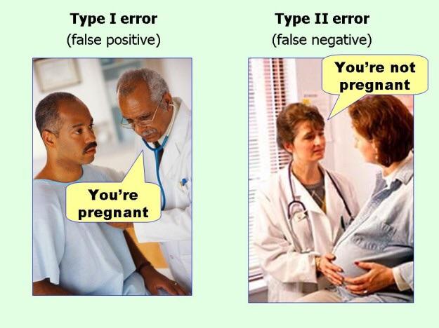
Figure 1. Type I and Type II errors.

Image credit: Ellis, P.D., “Effect Size FAQs,” accessed on January 10, 2018.

A Type II error, eloquently shown in Figure 1, is when the investigator (in this case the woman with the stethoscope expertly draped over her neck in the picture on the right) doesn’t detect an effect when an effect is there (it turns out this patient on the right is pregnant).

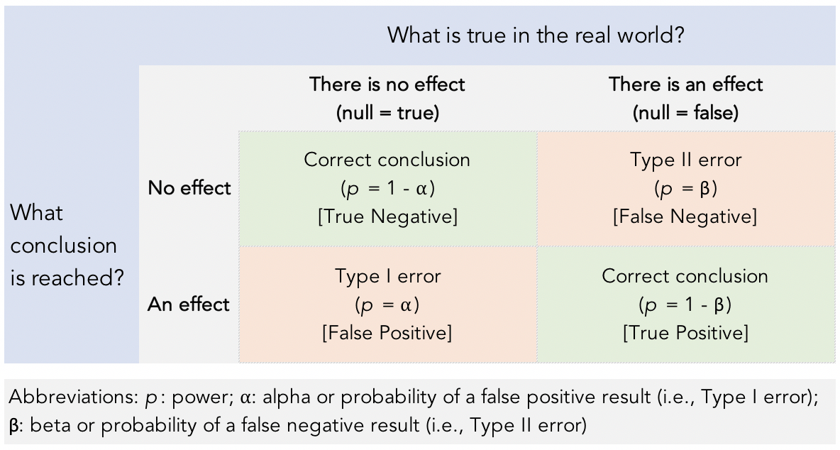
Figure 2. The four test outcomes.

What affects statistical power?

The power of any test of statistical significance will be affected by four things:

1. The probability of a false positive (Type I error) result (α)
2. The sample size (N)
3. The effect size (the magnitude of difference between groups)
4. The false negative (Type II) error rate (β)

Investigators designing a study use these four parameters to conduct a power analysis. You may have noticed that the effect size, is determined after the experiment. That’s the catch. If you’re an investigator running a power analysis, you’re probably doing it because you want to know how many subjects are required to adequately power your study. You can’t design an ironclad experiment without knowing the likely effect and you can’t know the effect until you’ve done the experiment.

How can an investigator better understand the size of the effect before the study? Reviewing the literature and the reported effect sizes of similar tests is a great place to start. The investigator should have a hypothesis going into the experiment, and that too should guide the determination. If possible, running a pre-test, or a pilot study is another way to get a better idea of how to power a larger experiment.

Alpha (α), if you recall, stands for the preselected significance level. Beta (β) is the chance of making a false negative (i.e., Type II error). Shooting for a 20 percent risk of β means designing studies such that they have an 80 percent probability of detecting real effects. The informal standard for an adequately powered study is 0.8. The investigator is conveying that if he or she performs the study flawlessly, it has a 1-in-5 chance of resulting in a false negative.

The sample size is the component that can easily over- or underpower a study. Many observational studies are arguably overpowered because they can have thousands to millions of subjects. Any small difference that gets picked up in such a study may yield a statistically significant result. Other studies may have the opposite issue. They may have a very small number of subjects, and relatively big differences between groups may not be statistically significant. (If you flip a fair coin five times and land on heads four times, and therefore observe a 30% absolute difference from the 50% mean—the coin landed on heads 80% of the time—you can probably understand why smaller samples need greater differences to be deemed statistically significant.)

Before we had online calculators, we had power tables. Nerd alert: in my spare time in residency I put together a General Surgery Review Manual that included a section on power analysis. In it, I used the following example to illustrate how to use a power table (Figure 3), “the single most important table for someone doing clinical research,” as my lab mentor, Steve Rosenberg, put it at the time:

“If, without intervention, the rate of an infection is 30%, and you expect your treatment to reduce it to 20%, you will require 411 patients per arm (822 in total) to have 90% power, or 313 per arm (626 in total) to have 80% power. To arrive at these numbers from the table below do the following: subtract the smaller success rate (0.20) from the larger success rate (0.30), 0.30 – 0.20 = 0.10. Align this column with the row corresponding to the smaller of the 2 success rates (in this example 0.20). This leads you to the numbers 411 and 313. The upper number is the number of subjects, per arm, required for 90% power, and the lower number the number of subjects, per arm, required for 80% power, with a significance of 95%. Glancing at this table from left to right you see that more subjects will be required when the expected difference between the treated and untreated groups is smaller. That is, the less of a difference the treatment is expected to have, the more subjects you will need to find a difference, should one exist.”  Of course, in real life, you would also bake in some buffer for drop out and determine if you need to do your analysis on a completion basis or intention-to-treat (ITT) basis.

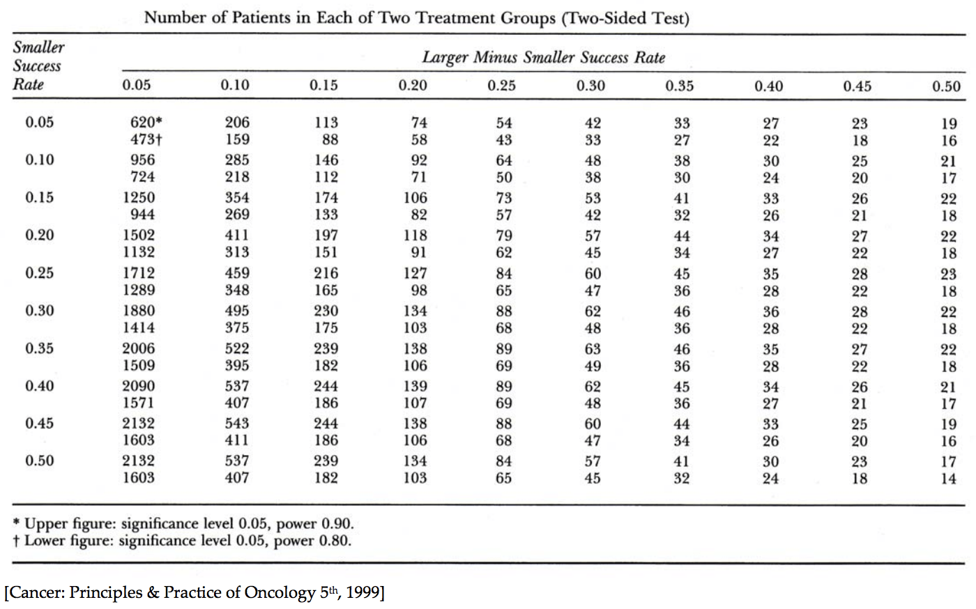
Figure 3. Power Table.

The art and science of power analysis is to balance how to insure against both Type I and Type II errors (with most of the insurance typically going toward Type I). All four parameters are mathematically related. If you know any three of them, you can figure out the fourth (Figure 4).

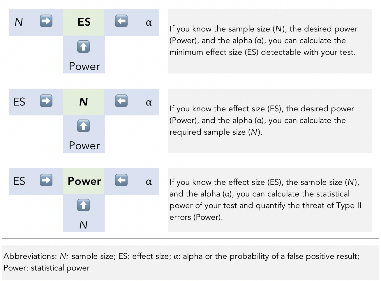
Figure 4. The relationship between the four parameters of power analysis.

Image adapted from Ellis, P.D., 2012. Statistical Power Trip.

Looking at the bottom example in Figure 4, we can answer the question we posed of a study that was not statistically significant: What magnitude of difference (i.e, effect size, or ES in the Figure) was the study powered to detect? We will know the three parameters after study completion and can plug it into an appropriate power and sample size calculator or consult a power table. This will help us get a better picture of the practical relevance of the study.

Full of sound and fury, signifying nothing (and occasionally, something)

One of the biggest take-home messages is that a study can be statistically significant, highly powered, with a high confidence level, but at the same time it can be practically insignificant, weak, and uncertain. The contrapositive can be true, too. Statistically weak studies may actually tell us something relatively powerful, and real, about the world around us.

Taken together, understanding statistical significance, p-values, power analysis, and confidence intervals can help one navigate the results of studies better, but it’s important to put them into context and understand that the meaningful information is not necessarily contained in a statistical vacuum.

§

We’ll pick up in a future installment summarizing what to look for, and perhaps more importantly, what to discard when confronted with the latest headlines and studies that are often imploring us to take notice.